ediblecity

library(ediblecity)

Set scenarios of urban agriculture

The function set_scenario provides a convenient way to create randomized scenarios for urban agriculture. We use the city_example provided with the package that is meant to serve as example to create a model for a city of interest.

We create one scenario, with 50% of normal gardens, vacant plot, streets and 75% of rooftops converted to edible_gardens. And with 50% of created gardens being for commercial purposes. To see the correspondence between original and urban agriculture elements, see ?set_scenario.

scenario <- set_scenario(city_example,
                           pGardens = 0.5,
                           pVacant = 0.5,
                           pRooftop = 0.75,
                           private_gardens_from = "Normal garden",
                           vacant_from = c("Vacant", "Streets"),
                           rooftop_from = "Rooftop",
                           pCommercial = 0.5)
#> Only 328 rooftops out of 453 assumed satisfy the 'min_area_rooftop'

The warnings are triggered when there are not elements enough to fulfill the proportions provided to the function.

in this examples, we use the scenario created with set_scenario, but all the indicators can be calculated using an sf object with the same structure as city_example.

Likewise, all the parameters used by the indicators are defined in city_land_uses. However, all indicators provide an option to override this an provide a customized dataframe with the parameters. The structure of this dataframe is detailed in the documentation of each function.

Estimate the benefits of urban agriculture

Urban Heat Island

The urban heat island indicator can return a summary of values or a stars object. It needs a raster representing the Sky view factor. See ?UHI for more details. We use the SVF object provided with the package.

withr::local_envvar(new = c("GTIFF_SRS_SOURCE" = "ESPG")) # To avoid CRS warning
UHI(scenario, SVF)
#>    Min. 1st Qu.  Median    Mean 3rd Qu.    Max. 
#>  0.0000  0.5465  1.0131  1.0298  1.4174  2.5867

withr::local_envvar(new = c("GTIFF_SRS_SOURCE" = "ESPG")) # To avoid CRS warning
plot(UHI(scenario, SVF, return_raster = TRUE))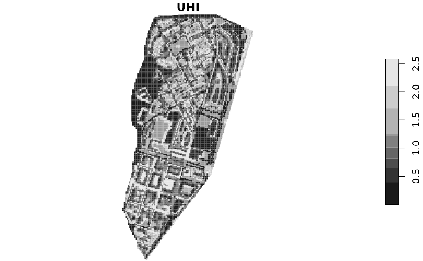

Runoff prevention

The function runoff_prev returns an estimation of the runoff in the city after a specific rain event (mm/day). It also estimates the total rainfall and the rainwater harvested by urban agriculture.

runoff_prev(scenario)
#>       runoff     rainfall  rainharvest 
#>     34.41038 108169.04500   1619.35446

Distance to closest green area

The function green_distance computes the distances from each home in the city to its closest public green area larger than a specific area. The homes must be identified using the column passed to residence_col. The default values for minimal area (0.5 ha) and for maximum distance (300 meters) follow the recommendations of WHO.

green_distance(scenario)
#>    Min. 1st Qu.  Median    Mean 3rd Qu.    Max. 
#>    6.12  155.08  251.70  249.72  347.42  465.73

If percent_out is set to TRUE, instead of a summary of distances, it returns the percentage of homes that are further than max_dist.

green_distance(scenario, percent_out = TRUE)
#> [1] 36.92615

Green per capita

The function green_capita calculates the amount of public and/or private green are per capita in the city. It can compute the total of the city, the values for each neighbourhood or the ratio between the neighbourhoods with minimum and maximum value (min / max).

green_capita(scenario, inhabitants = 6000)
#> [1] 10.81667

green_capita(scenario, 
             neighbourhoods = neighbourhoods_example, 
             inh_col = 'inhabitants',
             name_col = 'name',
             verbose = TRUE)
#> # A tibble: 2 × 4
#>   name              area inhabitants green_capita
#>   <chr>            <dbl>       <dbl>        <dbl>
#> 1 Sant Narcís nord 34916        1028        34.0 
#> 2 Sant Narcís sud  35064        5290         6.63

green_capita(scenario, 
             neighbourhoods = neighbourhoods_example, 
             inh_col = 'inhabitants',
             name_col = 'name')
#> [1] 0.1951526

Nitrogen dioxide (NO₂) sequestered by urban green

The function no2_seq computes the amount of NO₂ sequestered by urban green in gr/s.

no2_seq(scenario)
#>     gr/s 
#> 109.5444

Jobs created by commercial urban agriculture

The function edible_jobs estimates the number of jobs potentially created by commercial urban agriculture. Since the number of jobs / m2 is randomized, it computes a Monte Carlo simulation (n=1000) to estimate the value and returns the confidence interval (unless verbose = TRUE).

edible_jobs(scenario)
#>        5%       50%       95% 
#>  182.8589 1736.1195 3249.9924

Volunteers involved in community urban agriculture

The function edible_volunteers estimates the number of volunteers potentially involved in community urban agriculture. Since the number of volunteers / m2 is randomized, it computes a Monte Carlo simulation (n=1000) to estimate the value and returns the confidence interval (unless verbose = TRUE).

edible_volunteers(scenario)
#>        5%       50%       95% 
#>  259.8713 2363.1051 4468.8126

Food production

The function food_production estimates the food produced by urban agriculture (in kg/year). Since the productivity of each plot is randomized, It computes a Monte Carlo simulation (n=1000) to estimate the value and returns the confidence interval (unless verbose = TRUE).

food_production(scenario)
#>        5%       50%       95% 
#>  669965.8  918383.7 1150898.5

Randomization

The construction of scenarios as well as some parameters in the indicators are randomized to consider uncertainty. Our recommendation is to run each scenario you want to simulate in a Monte Carlo simulation to get the confidence interval for each indicator. You will find a practical implementation here.